Stellar Stream Fitting

This guide demonstrates three approaches to building a Track object for modeling stellar streams:

1. Direct construction from control points: When your data points are already well-suited as spline knots

2. Conversion from existing splines: When you have a spline fitted using other libraries (e.g., SciPy)—but beware of curvature issues

3. Optimization-based fitting: Advanced method that produces physically meaningful curvature for gravitational potential fitting

Each method is appropriate for different scenarios depending on your data quality and analysis requirements.

Method 1: Direct Construction from Control Points

When your data points are already of good quality and appropriately spaced, you can directly use them as control points for the spline. This is the simplest approach and requires minimal computation.

This method is ideal when:

• Data points are evenly distributed along the stream

• The number of points is reasonable (not too many, not too few)

• Points already capture the essential shape of the stream

Setup

import numpy as np
import matplotlib.pyplot as plt
import jax
import jax.numpy as jnp

# Enable 64-bit precision for better numerical accuracy
jax.config.update("jax_enable_x64", True)

import potamides as ptd
from potamides import splinelib

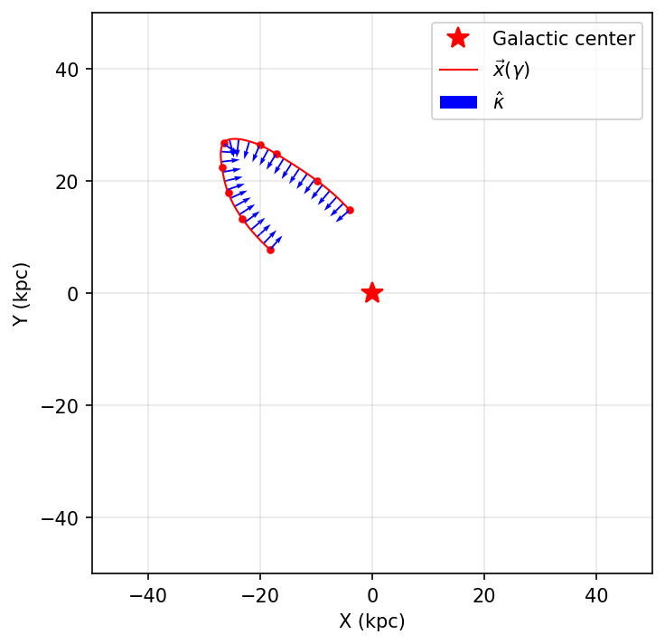
Example: Stream from Literature Data

# Example: manually extracted from Nibauer et al. (2023), Figure 5, second panel
stream_1 = np.array([[-18.23818192,   7.7713813 ],
                     [-23.20527332,  13.30501798],
                     [-25.68881901,  17.85818509],
                     [-26.82711079,  22.51483327],
                     [-26.51666758,  26.81189831],
                     [-20.04832301,  26.39824245],
                     [-17.02861664,  24.77713165],
                     [ -9.74451624,  19.97321842],
                     [ -4.03009244,  14.80896887]])

def make_gamma_from_data(data):
    """Compute normalized arc-length parameter gamma ∈ [-1, 1]"""
    s = splinelib.point_to_point_arclength(data)
    s = jnp.concat((jnp.array([0]), s))
    s_min = s.min()
    gamma = 2 * (s - s_min) / (s.max() - s_min) - 1
    return gamma

gamma = make_gamma_from_data(stream_1)
track = ptd.Track(gamma, stream_1)

Visualization

fig, ax = plt.subplots(figsize=(5, 5), dpi=150)
plt.plot(0, 0, 'r*', markersize=12, label='Galactic center')
plot_sparse_gamma = jnp.linspace(-1, 1, num=30)
track.plot_all(plot_sparse_gamma, ax=ax, show_tangents=False)
ax.set_xlabel("X (kpc)")
ax.set_ylabel("Y (kpc)")
ax.set_xlim(-50, 50)
ax.set_ylim(-50, 50)
ax.set_aspect('equal')
ax.legend()
ax.grid(alpha=0.3)
plt.tight_layout()
plt.show()

Method 2: Converting SciPy Splines to Track

Sometimes you may already have a spline fitted using other methods, such as SciPy’s UnivariateSpline. In this case, you can convert the scipy spline to a potamides.Track object to take advantage of additional features like computing tangent vectors, normal vectors, and curvature.

The conversion process involves:

1. Fitting separate univariate splines for X(γ) and Y(γ) using SciPy

2. Generating dense points along the fitted spline

3. Treating these dense points as new data points

4. Using jnp.column_stack to combine them into a JAX array

5. Computing arc-length parameterization with make_gamma_from_data

6. Creating the Track object with the re-parameterized gamma and points

Additional Setup

from scipy.interpolate import UnivariateSpline

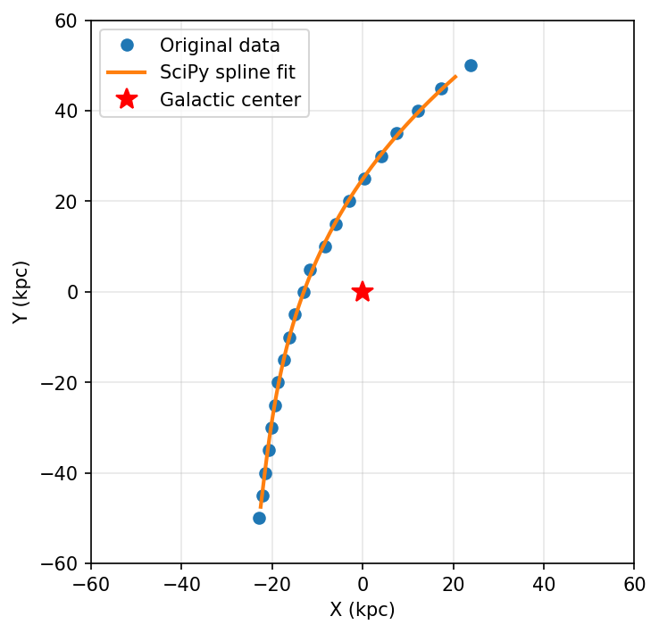
Fit a SciPy Spline

# Example data points for a curved stream
stream_2 = np.array([[ 23.8,  50. ],
                     [ 17.4,  45. ],
                     [ 12.1,  40. ],
                     [  7.5,  35. ],
                     [  4. ,  30. ],
                     [  0.4,  25. ],
                     [ -3. ,  20. ],
                     [ -6. ,  15. ],
                     [ -8.4,  10. ],
                     [-11.6,   5. ],
                     [-13. ,   0. ],
                     [-15. ,  -5. ],
                     [-16.3, -10. ],
                     [-17.4, -15. ],
                     [-18.8, -20. ],
                     [-19.4, -25. ],
                     [-20.2, -30. ],
                     [-20.8, -35. ],
                     [-21.6, -40. ],
                     [-22.2, -45. ],
                     [-23. , -50. ]])

# Extract X and Y coordinates
X = stream_2[:, 0]  # X coordinates (kpc)
Y = stream_2[:, 1]  # Y coordinates (kpc)
N = len(X)

# Create a parameterization gamma ∈ [-1, 1]
gamma = np.linspace(-1, 1, N)

# Fit univariate splines separately for X(gamma) and Y(gamma)
# k=3 for cubic spline, s=10 is the smoothing factor
cs_x = UnivariateSpline(gamma, X, k=3, s=10)
cs_y = UnivariateSpline(gamma, Y, k=3, s=10)

# Generate dense points along the spline for smooth visualization
# Note: Using restricted range [-0.95, 0.95] to avoid endpoint artifacts
gamma_new = np.linspace(-0.95, 0.95, 1000)
X_new = cs_x(gamma_new)
Y_new = cs_y(gamma_new)

Visualize SciPy Spline

fig, ax = plt.subplots(figsize=(5, 5), dpi=150)
plt.plot(X, Y, 'o', label='Original data', markersize=6)
plt.plot(X_new, Y_new, '-', label='SciPy spline fit', linewidth=2)
plt.plot(0, 0, 'r*', markersize=12, label='Galactic center')
plt.xlabel('X (kpc)')
plt.ylabel('Y (kpc)')
plt.xlim(-60, 60)
plt.ylim(-60, 60)
plt.gca().set_aspect('equal')
plt.legend()
plt.grid(alpha=0.3)
plt.tight_layout()
plt.show()

Convert to Potamides Track

The key insight here is that the dense points generated from the SciPy spline (X_new, Y_new) are treated as new data points. We combine them using jnp.column_stack to create a JAX array, then use the same make_gamma_from_data function to compute the arc-length parameterization.

# Convert the scipy spline to a potamides Track object

# Step 1: Combine X_new and Y_new into a 2D JAX array
# The dense points from scipy spline become our new "data points"
xy_for_track = jnp.column_stack([X_new, Y_new])

# Compute the arc-length parameterization gamma for the track
# This uses the same function as in Method 1, treating the dense points as data
gamma_track = make_gamma_from_data(xy_for_track)

# Step 2: Create the Track object
track_2 = ptd.Track(gamma_track, xy_for_track)

print(f"Track created successfully with {len(gamma_track)} points")
print(f"Gamma range: [{gamma_track.min():.3f}, {gamma_track.max():.3f}]")

Track created successfully with 1000 points
Gamma range: [-1.000, 1.000]

Visualize the Track

fig, ax = plt.subplots(figsize=(5, 5), dpi=150)

# Original data points
ax.plot(X, Y, 'o', label='Original data', alpha=0.6, markersize=6)

# Plot the potamides track
plot_sparse_gamma = jnp.linspace(-1, 1, num=30)
track_2.plot_all(plot_sparse_gamma, ax=ax, show_tangents=False)

ax.plot(0, 0, 'r*', markersize=12, label='Galactic center')
ax.set_xlabel('X (kpc)')
ax.set_ylabel('Y (kpc)')
ax.set_xlim(-60, 60)
ax.set_ylim(-60, 60)
ax.set_aspect('equal')
ax.legend()
ax.grid(alpha=0.3)
plt.tight_layout()
plt.show()

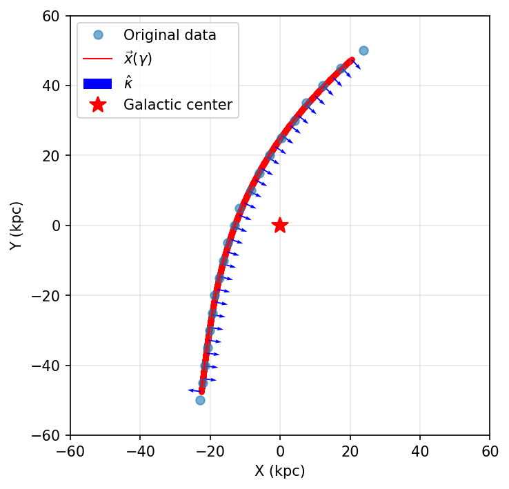
Limitations of Direct SciPy Conversion

As you can see in the visualization above, when splines are generated using standard fitting methods like SciPy’s UnivariateSpline, the curvature can sometimes be incorrect.

In this example, notice the lower end of the track (the bottom portion around y = -50 kpc): the curvature vectors point in a completely different direction than physically expected. This is a common issue because:

1. SciPy splines optimize for smooth interpolation, not physically meaningful curvature

2. The parameterization may not properly account for arc-length, leading to artificial variations in curvature

3. Endpoint effects can introduce spurious curvature that doesn’t reflect the true stream geometry

Why this matters for gravitational potential fitting: When using stream curvature to constrain gravitational potentials, incorrect curvature vectors will produce biased or incorrect parameter estimates. The curvature must accurately represent the gravitational acceleration field acting on the stream.

This problem motivated the development of the optimization-based approach in Method 3, which addresses these issues and produces tracks with physically consistent curvature throughout.

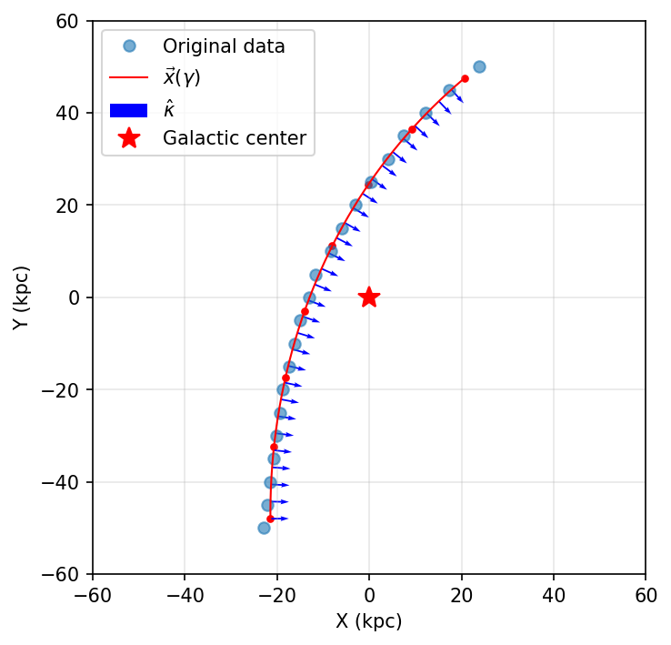
Method 3: Optimization-Based Fitting

To address the curvature issues seen in Method 2, we developed an optimization-based approach that produces physically meaningful tracks. This method:

1. Creates an initial fiducial spline directly from the data points

2. Optimizes the knot positions to minimize a cost function that enforces smooth, consistent curvature

3. Re-parameterizes gamma to be proportional to arc-length

4. Produces a smooth, well-behaved track suitable for gravitational potential fitting

Key advantage: Method 3 works directly with ordered data points—you don’t need to fit a SciPy spline first. The optimization process handles noisy or unevenly spaced data internally.

This method is ideal when:

• You need physically consistent curvature for scientific analysis (e.g., gravitational potential fitting)

• Data points are noisy or unevenly distributed

• You want fine control over the smoothness and complexity of the fit

• You need a specific number of knots for computational efficiency

Note: In this example, we use the same data (stream_2) as Method 2 to demonstrate how Method 3 produces better curvature. However, in practice, you would typically apply Method 3 directly to your ordered data points without the intermediate SciPy step.

Additional Setup

import interpax
from xmmutablemap import ImmutableMap

Adjusting Optimization Parameters

The splinelib.optimize_spline_knots function accepts several key parameters through cost_kwargs:

• sigmas: Uncertainty weights for each data point (default: 1.0)

• data_weight: Weight for the data fitting term, controls how closely the spline follows the data (default: 1e3)

• concavity_weight: Penalty for changes in curvature sign, enforces smoothness (default: 0.0)

• concavity_scale: Smoothing scale for the curvature penalty (default: 1e2)

In practice, you typically only need to adjust concavity_weight:

• Larger values (e.g., 1e10-1e12): Produce smoother curves with fewer inflection points

• Smaller values (e.g., 0-1e8): Allow more flexibility to fit local variations in the data

Start with a moderate value like 1e10 and increase it if the curve has unwanted wiggles, or decrease it if the curve is too smooth and misses important features.

The num_knots Parameter

Another critical parameter in make_optimal_track is num_knots, which determines the final track complexity:

• Too few knots: The fitted spline may differ significantly from the original data

• Too many knots: Can cause overfitting and produce incorrect curvature that cannot be fixed by adjusting cost_kwargs

In practice: Use num_knots between 5-15 and experiment to find the optimal value for your specific data

Optimization Function

def make_optimal_track(
    data: np.ndarray,
    /,
    *,
    num_knots: int,
    cost_kwargs: dict | None = None
) -> ptd.Track:
    """Create an optimal spline from data points.

    Parameters
    ----------
    data : np.ndarray
        Array of shape (N, 2) containing the (x, y) coordinates of the data points.
    num_knots : int
        Number of knots to use in the final optimized track.
    cost_kwargs : dict or None, optional
        Additional keyword arguments for the cost function, passed as an ImmutableMap.
        Common keys include:
        - 'concavity_weight': Penalty for changes in curvature sign (default: 1e10)
        - 'data_weight': Weight for data fitting term (default: 1e3)
        - 'sigmas': Uncertainty weights for each data point (default: 1.0)
        If None, defaults to {"concavity_weight": 1e10}.

    Returns
    -------
    ptd.Track
        The optimized track object.
    """
    # Set default cost_kwargs if not provided
    if cost_kwargs is None:
        cost_kwargs = {"concavity_weight": 1e10}

    # Create a fiducial spline from the data points
    fid_gamma, fid_knots = splinelib.make_increasing_gamma_from_data(data)
    fiducial_spline = interpax.Interpolator1D(fid_gamma, fid_knots, method="cubic2")

    # Evaluate the fiducial spline at a reference set of points at which to test
    # the spline during optimization
    ref_gamma = jnp.linspace(fid_gamma.min(), fid_gamma.max(), num=128)
    ref_points = fiducial_spline(ref_gamma)

    # Optimize the spline knots to minimize the cost function
    # Note: cost_kwargs must be converted to an ImmutableMap for JAX compatibility
    knots = splinelib.optimize_spline_knots(
        splinelib.default_cost_fn,
        fid_knots,
        fid_gamma,
        cost_args=(ref_gamma, ref_points),
        cost_kwargs=ImmutableMap(cost_kwargs),
    )
    # Create a spline from the optimized knots.
    spline = interpax.Interpolator1D(fid_gamma, knots, method="cubic2")

    # Create a new gamma, proportional to the arc-length from the spline.
    opt_gamma, opt_knots = splinelib.new_gamma_knots_from_spline(
        spline, nknots=num_knots
    )

    # Create the optimal track with the new gamma and optimized knots
    return ptd.Track(opt_gamma, opt_knots)

Create and Visualize the Optimized Track

# Create an optimal track directly from the original data points
# Note: We use stream_2 (the original ordered points) directly,
# not the SciPy-fitted points from Method 2
track_3 = make_optimal_track(stream_2, num_knots=8)

# Visualize the optimized track
fig, ax = plt.subplots(figsize=(5, 5), dpi=150)

# Original data points
ax.plot(X, Y, 'o', label='Original data', alpha=0.6, markersize=6)

# Plot the optimized potamides track
plot_sparse_gamma = jnp.linspace(-1, 1, num=30)
track_3.plot_all(plot_sparse_gamma, ax=ax, show_tangents=False)

ax.plot(0, 0, 'r*', markersize=12, label='Galactic center')
ax.set_xlabel('X (kpc)')
ax.set_ylabel('Y (kpc)')
ax.set_xlim(-60, 60)
ax.set_ylim(-60, 60)
ax.set_aspect('equal')
ax.legend()
ax.grid(alpha=0.3)
plt.tight_layout()
plt.show()

Summary

This guide covered three approaches to creating Track objects:

1. Direct construction is fastest and simplest when you have good quality control points that are already well-spaced

2. Conversion from SciPy enables integration with existing analysis pipelines, but may produce incorrect curvature (especially at endpoints)

3. Optimization-based fitting provides the most control and produces physically meaningful curvature for gravitational potential fitting

Recommended workflow:

• For well-spaced, clean data: Use Method 1 (direct construction)

• For noisy or unevenly spaced data: Use Method 3 (optimization) directly—no need to fit with SciPy first

• If you already have SciPy splines: You can convert them (Method 2), but be aware of potential curvature issues

Key comparison between Method 2 and Method 3:

• Method 2 (SciPy): Quick conversion if you already have SciPy splines, but may have incorrect curvature

• Method 3 (Optimization): Works directly with ordered data points, ensures physically consistent curvature throughout

• For gravitational potential fitting: Method 3 is strongly recommended as it produces reliable curvature vectors

Important: Method 3 does not require a SciPy spline as input—it works directly with your ordered (x, y) data points. The comparison in this tutorial simply demonstrates how Method 3 improves upon Method 2’s results when applied to the same data.