potamides library

`potamides` library#

API submodules

ptd.splinelib

potamides: Constrain gravitational potential with stream curvature

class potamides.AbstractTrack(ridge_line: Annotated[Interpolator1D, "[(N, F), method='cubic2']"])#

Bases: object

ABC for track classes.

It is strongly recommended to ensure that gamma is proportional to the arc-length of the track. A good definition of gamma is to normalize the arc-length to the range [-1, 1], such that

\[\gamma = \frac{2s}{L} - 1\]

where $s$ is the arc-length and $L$ is the total arc-length of the track.

Raises:: Exception – If the spline is not cubic2.

Examples

>>> import jax.numpy as jnp
>>> import potamides as ptd
>>> import matplotlib.pyplot as plt

>>> # Create a parametric circle with radius 2
>>> gamma = jnp.linspace(0, 2 * jnp.pi, 10_000)
>>> xy = 2 * jnp.stack([jnp.cos(gamma), jnp.sin(gamma)], axis=-1)
>>> track = ptd.Track(gamma, xy)

Basic position evaluation:

>>> gamma_test = jnp.array([0, jnp.pi / 2, jnp.pi])
>>> positions = track(gamma_test)
>>> print("Positions:", positions.round(2))
Positions: [[ 2.  0.]
            [ 0.  2.]
            [-2.  0.]]

Spherical coordinates (radius, angle):

>>> spherical = track.spherical_position(gamma_test)
>>> print("Spherical (r, theta):", spherical.round(4))
Spherical (r, theta): [[2.     0.    ]
                       [2.     1.5708]
                       [2.     3.1416]]

Tangent vectors along the track:

>>> tangents = track.tangent(gamma_test)
>>> print("Tangent vectors:", tangents.round(2))
Tangent vectors: [[ 0.  2.]
                  [-2.  0.]
                  [ 0. -2.]]

Curvature magnitude (for a circle, should be constant 1/radius):

>>> kappa_values = track.kappa(gamma_test)
>>> print("Curvature kappa:", kappa_values.round(4))
Curvature kappa: [0.5 0.5 0.5]

Curvature vectors:

>>> curvature_vecs = track.curvature(gamma_test)
>>> print("Curvature vectors:", curvature_vecs.round(2))
Curvature vectors: [[-0.5  0. ]
                    [ 0.  -0.5]
                    [ 0.5  0. ]]

Principal unit normal vectors (point toward center for circle):

>>> normals = track.principle_unit_normal(gamma_test)
>>> print("Unit normals:", normals.round(2))
Unit normals: [[-1.  0.]
               [ 0. -1.]
               [ 1.  0.]]

Access to track properties:

>>> print("Number of knots:", len(track.knots))
Number of knots: 10000
>>> print("Gamma range:", track.gamma.min().round(2), "to", track.gamma.max().round(2))
Gamma range: 0.0 to 6.28

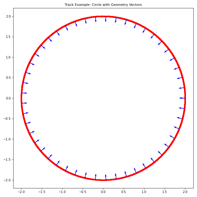
For visualization (requires matplotlib):

import jax.numpy as jnp
import potamides as ptd
import matplotlib.pyplot as plt

# Create a parametric circle with radius 2
gamma = jnp.linspace(0, 2 * jnp.pi, 10_000)
xy = 2 * jnp.stack([jnp.cos(gamma), jnp.sin(gamma)], axis=-1)
track = ptd.Track(gamma, xy)

# Create the plot
fig, ax = plt.subplots(figsize=(8, 8))
gamma_plot = jnp.linspace(0, 2*jnp.pi, 50)
track.plot_all(gamma_plot, ax=ax)
ax.set_aspect('equal')
ax.set_title('Track Example: Circle with Geometry Vectors')
plt.tight_layout()
plt.show()

acceleration(gamma: Real[Array, ''], /) → Real[Array, '2']#

Return the acceleration vector at a given position along the stream.

The acceleration vector is defined as: $\frac{d^2\vec{x}}{d\gamma^2}$.

Parameters:: gamma (Array[float, ()]) – The gamma value at which to evaluate the acceleration.
Returns:: The acceleration vector $\vec{a}$ at $\gamma$.
Return type:: Array[float, (N, 2)]

Examples

>>> import jax
>>> import jax.numpy as jnp
>>> import potamides as ptd

>>> gamma = jnp.linspace(0, 2 * jnp.pi, 10_000)
>>> xy = 2 * jnp.stack([jnp.cos(gamma), jnp.sin(gamma)], axis=-1)
>>> track = ptd.Track(gamma, xy)

>>> gamma = jnp.array([0, jnp.pi / 2, jnp.pi])
>>> acc = track.acceleration(gamma)
>>> print(acc.round(5))
[[-2.  0.]
 [ 0. -2.]
 [ 2.  0.]]

Return the arc-length of the track.

\[s(\gamma_0, \gamma_1) = \int_{\gamma_0}^{\gamma_1} \left\| \frac{d\mathbf{x}(\gamma)}{d\gamma} \right\| \, d\gamma\]

Computing the arc-length requires computing an integral over the norm of the tangent vector. This can be done using many different methods. We provide three options, specified by the method parameter.

Parameters:

gamma0 (float, optional) – The starting gamma value. Default is -1.
gamma1 (float, optional) – The ending gamma value. Default is 1.
method ({"p2p", "quad", "ode"}, optional) –
The method to use for computing the arc-length. Default is “p2p”.
- ”p2p”: point-to-point distance. This method computes the distance
  between each pair of points along the track and sums them up. Accuracy is limited by the 1e5 points used.
- ”quad”: quadrature. This method uses fixed quadrature to compute
  the integral. It is the default method. It also uses 1e5 points.
- ”ode”: ODE integration. This method uses ODE integration to compute the integral.
method_kw (dict, optional) – Additional keyword arguments to pass to the selected method.

curvature(gamma: Real[Array, ''], /) → Real[Array, '']#

Return the curvature at a given position along the stream.

This method computes the curvature by taking the ratio of the gamma derivative of the unit tangent vector to the derivative of the arc-length with respect to gamma. In other words, if

\[\frac{d\hat{T}}{d\gamma} = \frac{ds}{d\gamma} \frac{d\hat{T}}{ds}\]

and since the curvature vector is defined as

\[\frac{d\hat{T}}{ds} = \kappa \hat{N}\]

where $\kappa$ is the curvature and $\hat{N}$ the unit normal vector, then dividing $\frac{d\hat{T}}{d\gamma}$ by $\frac{ds}{d\gamma}$ yields

\[\kappa \hat{N} = \frac{d\hat{T}/d\gamma}{ds/d\gamma}\]

Here, $\frac{d\hat{T}}{d\gamma}$ (computed by dThat_dgamma) describes how the direction of the tangent changes with respect to the affine parameter $\gamma$, and $\frac{ds}{d\gamma}$ (obtained from state_speed) represents the state speed (i.e. the rate of change of arc-length with respect to $\gamma$).

This formulation assumes that $\gamma$ is chosen to be proportional to the arc-length of the track.

Parameters:: gamma (Array[float, ()]) – The gamma value at which to evaluate the curvature.
Returns:: The curvature vector $\kappa$ at $\gamma$.
Return type:: Array[float, (N, 2)]

Examples

>>> import jax
>>> import jax.numpy as jnp
>>> import potamides as ptd

>>> gamma = jnp.linspace(0, 2 * jnp.pi, 10_000)
>>> xy = 2 * jnp.stack([jnp.cos(gamma), jnp.sin(gamma)], axis=-1)
>>> track = ptd.Track(gamma, xy)

>>> gamma = jnp.array([0, jnp.pi / 2, jnp.pi])
>>> kappa = track.curvature(gamma)
>>> print(kappa.round(5))
[[-0.5  0. ]
 [ 0.  -0.5]
 [ 0.5  0. ]]

property gamma: Real[Array, 'N']#: Return the gamma values of the track.

kappa(gamma: Real[Array, ''], /) → Real[Array, '']#

Return the scalar curvature $\kappa(\gamma)$ along the track.

Parameters:: gamma (Array[float, ()]) – The gamma value at which to evaluate the curvature.
Returns:: The scalar curvature $\kappa$ at $\gamma$.
Return type:: Array[float, (N, 2)]

Examples

>>> import jax
>>> import jax.numpy as jnp
>>> import potamides as ptd

>>> gamma = jnp.linspace(0, 2 * jnp.pi, 10_000)
>>> xy = 2 * jnp.stack([jnp.cos(gamma), jnp.sin(gamma)], axis=-1)
>>> track = ptd.Track(gamma, xy)

>>> gamma = jnp.array([0, jnp.pi / 2, jnp.pi])
>>> kappa = track.kappa(gamma)
>>> print(kappa.round(5))
[0.5 0.5 0.5]

property knots: Real[Array, 'N F']#: Return the knot points along the track.

plot_all(gamma: Real[Array, 'N'], /, potential: AbstractPotential | None = None, *, ax: Axes | None = None, vec_width: float = 0.003, vec_scale: float = 30, labels: bool = True, show_tangents: bool = True, show_curvature: bool = True, track_kwargs: dict[str, Any] | None = None, curvature_kwargs: dict[str, Any] | None = None, acceleration_kwargs: dict[str, Any] | None = None) → Axes#

Plot the track, tangents, curvature, and local accelerations.

This method combines all the plotting methods into a single function to easily visualize the track, tangents, curvature, and local accelerations along the track. This is useful for quickly inspecting the geometry of a track.

Parameters:

gamma (Array[float, (N,)]) – The gamma values to evaluate the track and geometry at.
potential (galax.potential.AbstractPotential | None) – The potential to use for computing local accelerations. If None (default), the local acceleration vectors will not be plotted.
ax – The matplotlib.axes.Axes object to plot on. If None (default), a new figure and axes will be created.
vec_width – The width of the quiver arrows. Defaults to 0.003.
vec_scale – The scale factor for the quiver arrows. This affects the length of the arrows. Defaults to 30.
labels – Whether to show labels. Defaults to True.
show_tangents – Whether to plot the unit tangent vectors. Defaults to True.
show_curvature – Whether to plot the unit curvature vectors. Defaults to True.
track_kwargs (dict, optional) – Additional keyword arguments to pass to the track plotting method.
curvature_kwargs (dict, optional) – Additional keyword arguments to pass to the curvature plotting method.
acceleration_kwargs (dict, optional) – Additional keyword arguments to pass to the acceleration plotting method.

Returns:

The matplotlib axes containing the complete plot.

Return type:

matplotlib.axes.Axes

Examples

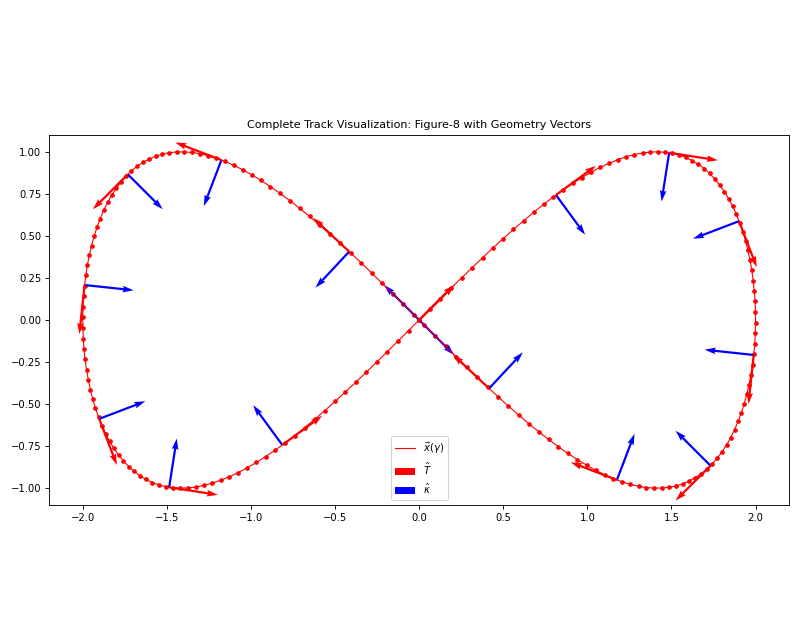
Basic track visualization with geometry vectors:

import jax.numpy as jnp
import potamides as ptd
import matplotlib.pyplot as plt

# Create a figure-8 track for interesting geometry
gamma = jnp.linspace(0, 2 * jnp.pi, 200)
x = 2 * jnp.sin(gamma)
y = jnp.sin(2 * gamma)
xy = jnp.stack([x, y], axis=-1)
track = ptd.Track(gamma, xy)

# Plot all geometric features
fig, ax = plt.subplots(figsize=(10, 8))
gamma_vectors = jnp.linspace(0, 2*jnp.pi, 16)

track.plot_all(gamma_vectors, ax=ax, vec_scale=15)
ax.set_aspect('equal')
ax.set_title('Complete Track Visualization: Figure-8 with Geometry Vectors')
ax.legend()
plt.tight_layout()
plt.show()

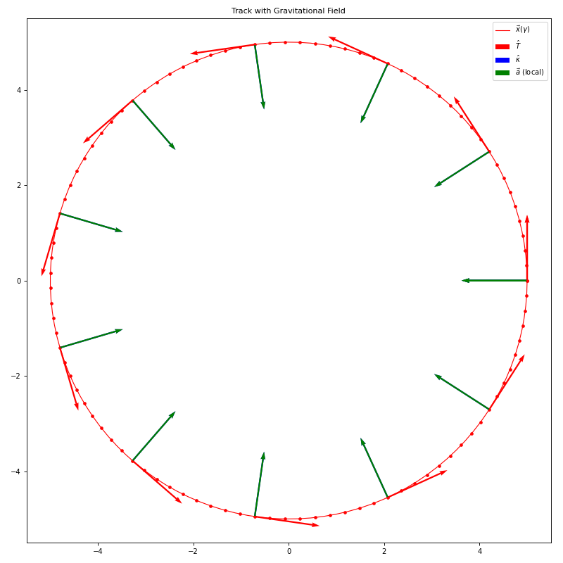
Track with gravitational potential:

import jax.numpy as jnp
import potamides as ptd
import galax.potential as gp
import matplotlib.pyplot as plt

# Create a circular track
gamma = jnp.linspace(0, 2 * jnp.pi, 100)
xy = 5 * jnp.stack([jnp.cos(gamma), jnp.sin(gamma)], axis=-1)
track = ptd.Track(gamma, xy)

# Add a gravitational potential
potential = gp.KeplerPotential(m_tot=1e12, units="galactic")

# Plot everything including gravitational field
fig, ax = plt.subplots(figsize=(10, 10))
gamma_vectors = jnp.linspace(0, 2*jnp.pi, 12)

track.plot_all(gamma_vectors, potential=potential, ax=ax, vec_scale=8)
ax.set_aspect('equal')
ax.set_title('Track with Gravitational Field')
ax.legend()
plt.tight_layout()
plt.show()

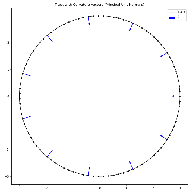
plot_curvature(gamma: Real[Array, 'N'], *, ax: Axes | None = None, vec_width: float = 0.003, vec_scale: float = 30, color: str = 'blue', label: str | None = '$\\hat{\\kappa}$') → Axes#

Plot the principal unit normal vectors along the track.

This method visualizes the principal unit normal vectors at specified points along the track. These vectors point in the direction of curvature and are perpendicular to the tangent vectors, showing how the track curves.

Parameters:

gamma (Array[float, (N,)]) – The gamma values where normal vectors will be plotted.
ax – The matplotlib axes to plot on. If None (default), creates a new figure.
vec_width – The width of the quiver arrows. Default is 0.003.
vec_scale – The scale factor for arrow lengths (higher = shorter arrows). Default is 30.
color – The color of the normal vector arrows. Default is “blue”.
label – The label for the normal vectors in the legend. If None (default), no label is added. Default is r”$\hat{\kappa}$”.

Returns:

The matplotlib axes containing the plot.

Return type:

matplotlib.axes.Axes

Examples

import jax.numpy as jnp
import potamides as ptd
import matplotlib.pyplot as plt

# Create a circular track
gamma = jnp.linspace(0, 2 * jnp.pi, 100)
xy = 3 * jnp.stack([jnp.cos(gamma), jnp.sin(gamma)], axis=-1)
track = ptd.Track(gamma, xy)

# Plot track with curvature vectors
fig, ax = plt.subplots(figsize=(8, 8))
gamma_plot = jnp.linspace(0, 2*jnp.pi, 200)
gamma_vectors = jnp.linspace(0, 2*jnp.pi, 12)

track.plot_track(gamma_plot, ax=ax, c='black', label='Track')
track.plot_curvature(gamma_vectors, ax=ax, color='blue', vec_scale=20)

ax.set_aspect('equal')
ax.set_title('Track with Curvature Vectors (Principal Unit Normals)')
ax.legend()
plt.tight_layout()
plt.show()

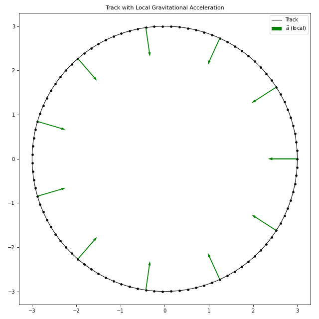
plot_local_accelerations(potential: AbstractPotential, gamma: Real[Array, 'N'], /, t: float = 0, *, vec_width: float = 0.003, vec_scale: float = 30, ax: Axes | None = None, label: str | None = '$\\vec{a}$ (local)', color: str = 'green') → Axes#

Plot the local gravitational acceleration vectors along the track.

This method visualizes the gravitational acceleration vectors from a given potential at specified points along the track. This is useful for understanding how the gravitational field affects the motion along the track.

potentialgalax.potential.AbstractPotential
The gravitational potential to evaluate accelerations.

gammaArray[float, (N,)]
The gamma values where acceleration vectors will be plotted.

t
The time at which to evaluate the potential (for time-dependent potentials). Defaults to 0.

vec_width
The width of the quiver arrows. Defaults to 0.003.

vec_scale
The scale factor for arrow lengths (higher = shorter arrows). Defaults to 30.

ax
The matplotlib axes to plot on. If None (default), creates a new figure.

label
The label for the acceleration vectors in the legend. If None, no label is added. Defaults to ``r”$

ec{a}$ (local)”``.

color: The color of the acceleration vector arrows. Defaults to “green”.

matplotlib.axes.Axes: The matplotlib axes containing the plot.

Track with gravitational potential:

import jax.numpy as jnp
import potamides as ptd
import galax.potential as gp
import matplotlib.pyplot as plt

# Create a circular track
gamma = jnp.linspace(0, 2 * jnp.pi, 100)
xy = 3 * jnp.stack([jnp.cos(gamma), jnp.sin(gamma)], axis=-1)
track = ptd.Track(gamma, xy)

# Create a simple point mass potential at origin
potential = gp.KeplerPotential(m_tot=1e12, units="galactic")

# Plot track with local acceleration vectors
fig, ax = plt.subplots(figsize=(8, 8))
gamma_plot = jnp.linspace(0, 2*jnp.pi, 200)
gamma_vectors = jnp.linspace(0, 2*jnp.pi, 12)

track.plot_track(gamma_plot, ax=ax, c='black', label='Track')
track.plot_local_accelerations(potential, gamma_vectors, ax=ax,
                              color='green', vec_scale=10)

ax.set_aspect('equal')
ax.set_title('Track with Local Gravitational Acceleration')
ax.legend()
plt.tight_layout()
plt.show()

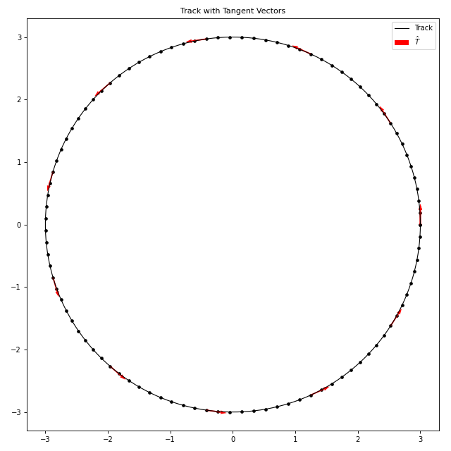
plot_tangents(gamma: Real[Array, 'N'], *, ax: Axes | None = None, vec_width: float = 0.003, vec_scale: float = 30, color: str = 'red', label: str | None = '$\\hat{T}$') → Axes#

Plot the unit tangent vectors along the track.

This method visualizes the normalized tangent vectors at specified points along the track. The tangent vectors show the direction of motion along the parametric curve.

Parameters:

gamma (Array[float, (N,)]) – The gamma values where tangent vectors will be plotted.
ax – The matplotlib axes to plot on. If None (default), creates a new figure.
vec_width – The width of the quiver arrows. Default is 0.003.
vec_scale – The scale factor for arrow lengths (higher = shorter arrows). Default is 30.
color – The color of the tangent vector arrows. Default is “red”.
label – The label for the tangent vectors in the legend. If None, no label is added. Default is r”$\hat{T}$”.

Returns:

The matplotlib axes containing the plot.

Return type:

matplotlib.axes.Axes

Examples

import jax.numpy as jnp
import potamides as ptd
import matplotlib.pyplot as plt

# Create a circular track
gamma = jnp.linspace(0, 2 * jnp.pi, 100)
xy = 3 * jnp.stack([jnp.cos(gamma), jnp.sin(gamma)], axis=-1)
track = ptd.Track(gamma, xy)

# Plot track with tangent vectors
fig, ax = plt.subplots(figsize=(8, 8))
gamma_plot = jnp.linspace(0, 2*jnp.pi, 200)
gamma_vectors = jnp.linspace(0, 2*jnp.pi, 12)

track.plot_track(gamma_plot, ax=ax, c='black', label='Track')
track.plot_tangents(gamma_vectors, ax=ax, color='red', vec_scale=20)

ax.set_aspect('equal')
ax.set_title('Track with Tangent Vectors')
ax.legend()
plt.tight_layout()
plt.show()

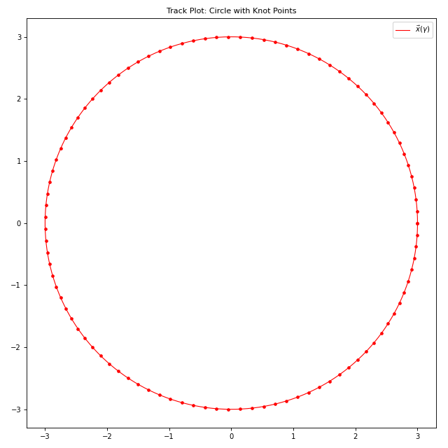
plot_track(gamma: Real[Array, 'N'], /, *, ax: Axes | None = None, label: str | None = '$\\vec{x}$($\\gamma$)', c: str = 'red', ls: str = '-', lw: float = 1.0, l_zorder: int = 2, knot_size: int = 10, knot_zorder: int = 1) → Axes#

Plot the track curve itself with knot points.

This method visualizes the parametric track curve as a continuous line and overlays the knot points used in the spline interpolation.

Parameters:

gamma (Array[float, (N,)]) – The gamma values to evaluate and plot the track at.
ax (plt.Axes, optional) – The matplotlib axes to plot on. If None, creates a new figure.
label (str, optional) – The label for the track curve in the legend.
c (str, default "red") – The color for the track curve and knot points.
ls (str, default "-") – The line style for the track curve.
lw (float, default 1.0) – The line width for the track curve.
l_zorder (int, default 2) – The z-order for the track line (controls layering).
knot_size (int, default 10) – The size of the knot point markers.
knot_zorder (int, default 1) – The z-order for the knot points (controls layering).

Returns:

The matplotlib axes containing the plot.

Return type:

matplotlib.axes.Axes

Examples

import jax.numpy as jnp
import potamides as ptd
import matplotlib.pyplot as plt

# Create a circular track
gamma = jnp.linspace(0, 2 * jnp.pi, 100)
xy = 3 * jnp.stack([jnp.cos(gamma), jnp.sin(gamma)], axis=-1)
track = ptd.Track(gamma, xy)

# Plot just the track
fig, ax = plt.subplots(figsize=(8, 8))
gamma_plot = jnp.linspace(0, 2*jnp.pi, 200)
track.plot_track(gamma_plot, ax=ax)
ax.set_aspect('equal')
ax.set_title('Track Plot: Circle with Knot Points')
ax.legend()
plt.tight_layout()
plt.show()

positions(gamma: Real[Array, 'N']) → Real[Array, 'N 2']#

Return the position at a given gamma.

Examples

Compute the position for specific points on the unit circle:

>>> import jax.numpy as jnp
>>> import interpax
>>> import potamides as ptd

>>> gamma = jnp.linspace(0, 2 * jnp.pi, 10_000)
>>> xy = 2  * jnp.stack([jnp.cos(gamma), jnp.sin(gamma)], axis=-1)
>>> track = ptd.Track(gamma, xy)

>>> gamma = jnp.array([0, jnp.pi / 2, jnp.pi])
>>> print(track.positions(gamma).round(2))
[[ 2.  0.]
 [ 0.  2.]
 [-2.  0.]]

principle_unit_normal(gamma: Real[Array, ''], /) → Real[Array, '2']#

Return the unit normal vector at a given position along the stream.

The unit normal vector is defined as the normalized acceleration vector:

\[\hat{N} = \frac{d^2\vec{x}/d\gamma^2}{\left\| d^2\vec{x}/d\gamma^2 \right\|}\]

Parameters:: gamma (Array[float, ()]) – The gamma value at which to evaluate the normal vector.
Returns:: The unit normal vector $\hat{N}$ at $\gamma$.
Return type:: Array[float, (N, 2)]

Examples

>>> import jax
>>> import jax.numpy as jnp
>>> import potamides as ptd

>>> gamma = jnp.linspace(0, 2 * jnp.pi, 10_000)
>>> xy = 2 * jnp.stack([jnp.cos(gamma), jnp.sin(gamma)], axis=-1)
>>> track = ptd.Track(gamma, xy)

>>> gamma = jnp.array([0, jnp.pi / 2, jnp.pi])
>>> Nhat = track.principle_unit_normal(gamma)
>>> print(Nhat.round(5))
[[-1.  0.]
 [ 0. -1.]
 [ 1.  0.]]

ridge_line: Annotated[Interpolator1D, "[(N, F), method='cubic2']"]#

The spline interpolator for the track, parametrized by gamma.

This must be twice-differentiable (cubic2) to enable computation of curvature vectors and other second-order geometric properties.

spherical_position(gamma: Real[Array, 'N'], /) → Real[Array, 'N 2']#

Compute $|\vec{f}(gamma)|$ at $\gamma$.

Examples

>>> import jax.numpy as jnp
>>> import potamides as ptd

>>> gamma = jnp.linspace(0, 2 * jnp.pi, 10_000)
>>> xy = 2 * jnp.stack([jnp.cos(gamma), jnp.sin(gamma)], axis=-1)
>>> track = ptd.Track(gamma, xy)

>>> gamma = jnp.array([0, jnp.pi / 2, jnp.pi])
>>> r = track.spherical_position(gamma)
>>> print(r.round(4))
[[2.     0.    ]
 [2.     1.5708]
 [2.     3.1416]]

state_speed(gamma: Real[Array, ''], /) → Real[Array, '']#

Return the speed in gamma of the track at a given position.

This is the norm of the tangent vector at the given position.

\[\mathbf{v}(\gamma) = \left\| \frac{d\mathbf{x}(\gamma)}{d\gamma} \right\|\]

An important note is that this is also equivalent to the derivative of the arc-length with respect to gamma.

On a 2D flat surface (the flat-sky approximation is reasonable for observations of extragalactic stellar streams) the differential arc-length is given by:

\[s = \int_{\gamma_0}^{\gamma} \sqrt{\left(\frac{dx}{d\gamma}\right)^2 + \left(\frac{dy}{d\gamma}\right)^2} d\gamma\]

Thus, the arc-length element is:

\[\frac{ds}{d\gamma} = \sqrt{\left(\frac{dx}{d\gamma}\right)^2 + \left(\frac{dy}{d\gamma}\right)^2}\]

If $\gamma$ is proportional to the arc-length, which is a very good and common choice, then for $\gamma \in [-1, 1] = \frac{2s}{L} - 1$, we have

\[\frac{ds}{d\gamma} = \frac{L}{2}\]

where $L$ is the total arc-length of the stream.

Since this is a constant, there is no need to compute this function. It is sufficient to just use $L/2$. This function is provided for completeness.

Parameters:: gamma (Array[float, ()]) – The gamma value at which to evaluate the spline.

tangent(gamma: Real[Array, ''], /) → Real[Array, '2']#

Compute the tangent vector at a given position along the stream.

The tangent vector is defined as:

\[T(\gamma) = \frac{d\vec{x}}{d\gamma}\]

Parameters:: gamma (Array[float, ()]) – The gamma value at which to evaluate the spline.
Returns:: The tangent vector at the specified position.
Return type:: Array[real, (*batch, 2)]

Examples

Compute the tangent vector for specific points on the unit circle:

>>> import jax.numpy as jnp
>>> import interpax
>>> import potamides as ptd

>>> gamma = jnp.linspace(0, 2 * jnp.pi, 10_000)
>>> x = 2 * jnp.cos(gamma)
>>> y = 2 * jnp.sin(gamma)
>>> track = ptd.Track(gamma, jnp.stack([x, y], axis=-1))

>>> gamma = jnp.array([0, jnp.pi / 2, jnp.pi])
>>> tangents = track.tangent(gamma)
>>> print(tangents.round(2))
[[ 0.  2.]
 [-2.  0.]
 [ 0. -2.]]

property total_arc_length: Real[Array, '']#

Return the total arc-length of the track.

\[L = s(-1, 1) = \int_{-1}^{1} \left\| \frac{d\mathbf{x}(\gamma)}{d\gamma} \right\| \, d\gamma\]

This is equivalent to arc_length with gamma0=-1 and gamma1=1. The method used is the default method, which is “quad”.

class potamides.Track(gamma: Real[Array, 'gamma'] | None = None, knots: Real[Array, 'gamma F'] | None = None, /, *, ridge_line: Interpolator1D | None = None)#

Bases: AbstractTrack

Concrete implementation of a parametric track using spline interpolation.

This class represents a smooth parametric curve in 2D space using cubic spline interpolation. It provides a concrete implementation of the AbstractTrack interface with automatic spline construction from data points or direct spline specification.

The track is parameterized by gamma values and uses cubic2 spline interpolation to ensure twice-differentiability, which is required for computing curvature vectors and other geometric properties.

Parameters:

gamma (Array[float, (N,)]) – The parameter values along the track. Must be provided together with knots if ridge_line is not specified.
knots (Array[float, (N, F)]) – The position data points corresponding to gamma values, where F is the spatial dimension (typically 2 for x,y coordinates). Must be provided together with gamma if ridge_line is not specified.
ridge_line (interpax.Interpolator1D) – Pre-constructed spline interpolator. If provided, gamma and knots must be None.

Raises:

ValueError – If neither (gamma, knots) nor ridge_line is provided, or if both are provided simultaneously.
ValueError – If the spline method is not “cubic2” (required for curvature computation).

Examples

Create a circular track from parametric data:

>>> import jax.numpy as jnp
>>> import potamides as ptd

>>> # Generate circle data
>>> gamma = jnp.linspace(0, 2 * jnp.pi, 100)
>>> x = 3 * jnp.cos(gamma)
>>> y = 3 * jnp.sin(gamma)
>>> knots = jnp.stack([x, y], axis=-1)
>>> track = ptd.Track(gamma, knots)

>>> # Evaluate track at specific points
>>> test_gamma = jnp.array([0, jnp.pi/2, jnp.pi])
>>> positions = track(test_gamma)
>>> print("Positions:", positions.round(2))
Positions: [[ 3.  0.]
            [ 0.  3.]
            [-3.  0.]]

Create a sinusoidal track:

>>> gamma = jnp.linspace(-1, 1, 50)
>>> x = gamma
>>> y = jnp.sin(3 * jnp.pi * gamma)
>>> knots = jnp.stack([x, y], axis=-1)
>>> track = ptd.Track(gamma, knots)

>>> # Compute geometric properties
>>> gamma_test = jnp.array([-0.5, 0, 0.5])
>>> tangents = track.tangent(gamma_test)
>>> curvatures = track.kappa(gamma_test)
>>> print("Curvatures:", curvatures.round(3))
Curvatures: [88.684  0.    88.684]

Create from an existing spline:

>>> import interpax
>>> gamma = jnp.linspace(0, 1, 20)
>>> y = gamma**2
>>> knots = jnp.stack([gamma, y], axis=-1)
>>> spline = interpax.Interpolator1D(gamma, knots, method="cubic2")
>>> track = ptd.Track(ridge_line=spline)

Track properties and methods:

>>> print("Gamma range:", track.gamma.min(), "to", track.gamma.max())
Gamma range: 0.0 to 1.0
>>> print("Number of knots:", len(track.knots))
Number of knots: 20
>>> arc_length = track.total_arc_length
>>> print("Total arc length:", arc_length.round(3))
Total arc length: 1.479

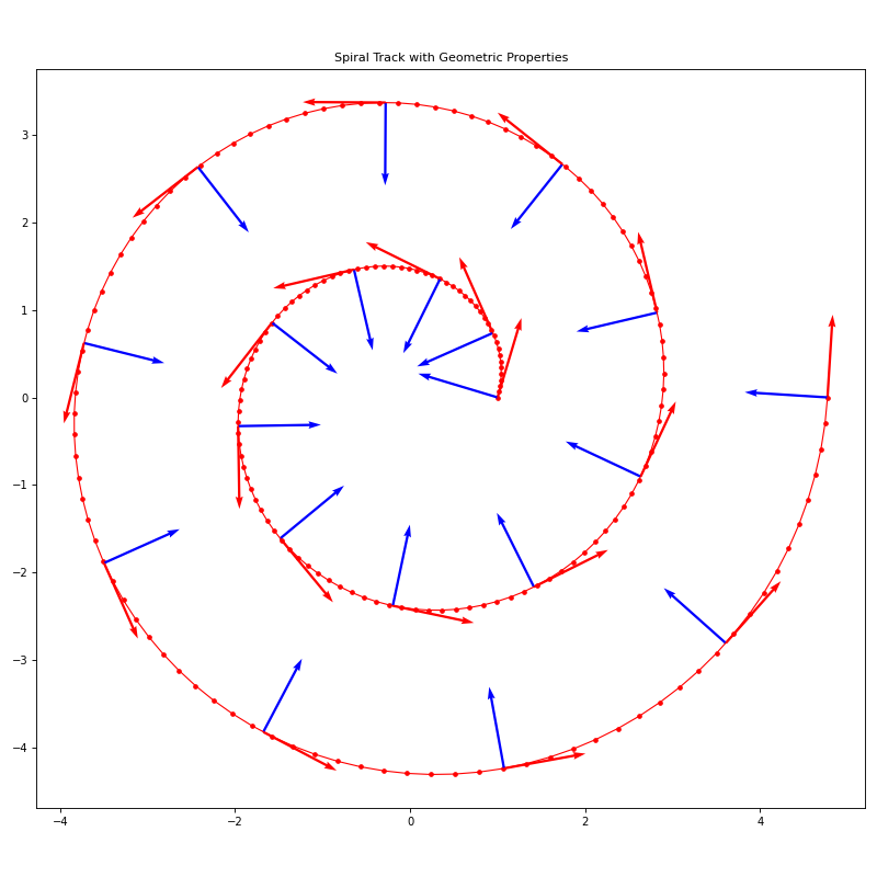
Visualization example:

import jax.numpy as jnp
import potamides as ptd
import matplotlib.pyplot as plt

# Create a spiral track
gamma = jnp.linspace(0, 4*jnp.pi, 200)
r = 1 + 0.3 * gamma
x = r * jnp.cos(gamma)
y = r * jnp.sin(gamma)
knots = jnp.stack([x, y], axis=-1)
track = ptd.Track(gamma, knots)

# Plot the track with geometric vectors
fig, ax = plt.subplots(figsize=(10, 10))
gamma_plot = jnp.linspace(0, 4*jnp.pi, 400)
gamma_vectors = jnp.linspace(0, 4*jnp.pi, 20)

track.plot_all(gamma_vectors, ax=ax, vec_scale=10)
ax.set_aspect('equal')
ax.set_title('Spiral Track with Geometric Properties')
plt.tight_layout()
plt.show()

See also

AbstractTrack: Base class defining the track interface
interpax.Interpolator1D: The underlying spline interpolation class

Notes

The Track class is designed to work seamlessly with JAX transformations including jit compilation, automatic differentiation, and vectorization. All geometric computations are performed using JAX operations for optimal performance.

The spline interpolation uses the “cubic2” method which ensures the track is twice-differentiable everywhere, enabling computation of curvature vectors and higher-order geometric properties.

classmethod from_spline(spline: Interpolator1D, /) → Track#

Create a Track from an existing spline interpolator.

Parameters:: spline (interpax.Interpolator1D) – An existing spline interpolator that will be used as the ridge_line for the track. The spline must use the “cubic2” method to ensure twice-differentiability for curvature computations.
Returns:: A new Track instance using the provided spline as its ridge_line.
Return type:: Track
Raises:: ValueError – If the spline method is not “cubic2”, which is required for computing curvature vectors and other second-order geometric properties.

Examples

>>> import jax.numpy as jnp
>>> import interpax
>>> import potamides as ptd

>>> gamma = jnp.linspace(-2, 2, 50)
>>> knots = jnp.stack([gamma, gamma**2], axis=-1)

>>> spline = interpax.Interpolator1D(gamma, knots, method="cubic2")

>>> track = ptd.Track.from_spline(spline)

potamides.combine_ln_likelihoods(lnliks: Real[Array, 'S'], /, ngammas: Int[Array, 'S'], arclengths: Real[Array, 'S']) → Real[Array, '']#

Combine likelihoods from different stream segments with density weighting.

This function combines log-likelihoods from multiple stream segments by applying density-based weighting. Stream segments with lower measurement density (fewer gamma points per unit arc-length) are up-weighted, while segments with higher measurement density are down-weighted. This ensures fair contribution from all segments regardless of their sampling density.

The function is vectorized using JAX’s jnp.vectorize with signature (n),(n),(n)->(), allowing it to process multiple sets of stream segments in parallel. When given 2D input arrays, it processes each row independently and returns a 1D array of combined likelihoods.

Parameters:

lnliks (Array[float, (S,)]) – The log-likelihoods of S stream segments. For vectorized operation, this can be a 2D array where each row represents a different set of stream segments.
ngammas (Array[int, (S,)]) – The number of gamma points in each of the S stream segments. Must have the same shape as lnliks.
arclengths (Array[float, (S,)]) – The total arc-lengths of the S stream segments. Must have the same shape as lnliks.

Returns:

The combined weighted log-likelihood. For vectorized inputs, returns an array with one combined likelihood per input set.

Return type:

Array[float, ()]

Notes

The weighting scheme computes the mean measurement density across all segments and uses this to normalize individual segment contributions:

\[ \begin{align}\begin{aligned}\bar{\rho} = \frac{\sum_i n_i}{\sum_i L_i}\\w_i = \frac{\bar{\rho}}{\rho_i} = \frac{\bar{\rho} L_i}{n_i}\\\mathcal{L}_{combined} = \sum_i w_i \mathcal{L}_i\end{aligned}\end{align} \]

where $n_i$ is the number of gamma points, $L_i$ is the arc-length, and $\mathcal{L}_i$ is the log-likelihood for segment $i$.

Examples

>>> import jax.numpy as jnp
>>> import potamides as ptd

>>> # Scalar inputs - single set of stream segments
>>> lnliks = jnp.array([0.5, 1.0, 1.5])
>>> ngammas = jnp.array([100, 100, 100])
>>> arclengths = jnp.array([1.0, 1.0, 1.0])
>>> combined = ptd.combine_ln_likelihoods(lnliks, ngammas, arclengths)
>>> print(combined)
3.0

>>> # Vector inputs - multiple sets of stream segments
>>> lnliks = jnp.array([[0.1, 0.2, 0.3], [0.4, 0.5, 0.6]])
>>> ngammas = jnp.array([[100, 200, 300], [150, 250, 350]])
>>> arclengths = jnp.array([[1.0, 2.0, 3.0], [1.5, 2.5, 3.5]])
>>> combined = ptd.combine_ln_likelihoods(lnliks, ngammas, arclengths)
>>> print(combined.round(1))
[0.6 1.5]

Calculate the planar acceleration (x-y plane, ignoring the z-component along the line-of-sight direction) at each given position.

The gravitational potentials are modeled using two types: a Logarithmic potential for the halo and a Miyamoto-Nagai potential for the disk, if included.

Parameters:

pos – An array of shape (N, 3) where N is the number of positions. Each position is a 3D coordinate (x, y, z) in kpc.
rot_z – Rotation angle [radians] around the z-axis (applied first). Default 0.0.
rot_x – Rotation angle [radians] around the x-axis (applied second). Default 0.0.
q1 – Halo axis ratios for the logarithmic potential. q1 and q2 control flattening in the x-y plane, q3 controls flattening along z-axis. Default 1.0.
q2 – Halo axis ratios for the logarithmic potential. q1 and q2 control flattening in the x-y plane, q3 controls flattening along z-axis. Default 1.0.
q3 – Halo axis ratios for the logarithmic potential. q1 and q2 control flattening in the x-y plane, q3 controls flattening along z-axis. Default 1.0.
phi – Orientation angle [radians] of the halo potential. Default 0.0.
rs_halo – Halo scale radius [kpc]. Default 16.0 kpc.
vc_halo – Halo circular velocity. Default 250 km/s converted to kpc/Myr.
origin – Halo center coordinates [kpc]. Default [0, 0, 0].
Mdisk – Disk mass [Msun]. Only used if withdisk is True. Default 1.2e10.
withdisk – If True, include a Miyamoto-Nagai disk potential in addition to the halo. Default False.

Returns:

An array of shape (N, 2) representing the planar (x-y) acceleration unit vectors at each input position.

Return type:

Array[float, (N, 2)]

Examples

>>> import jax.numpy as jnp
>>> import numpy as np
>>> import unxt as u
>>> import potamides as ptd

>>> # Basic usage: compute accelerations at a few positions
>>> positions = jnp.array([
...     [8.0, 0.0, 0.0],    # Solar neighborhood
...     [0.0, 8.0, 0.0],    # 90 degrees around
...     [4.0, 4.0, 1.0],    # Inner galaxy, off-plane
... ])
>>> acc_xy = ptd.compute_accelerations(positions)
>>> print(f"Shape: {acc_xy.shape}")
Shape: (3, 2)
>>> print(f"All finite: {jnp.all(jnp.isfinite(acc_xy))}")
All finite: True

>>> # Using quantities with units
>>> pos_with_units = u.Quantity([8.0, 0.0, 0.0], "kpc").reshape(1, 3)
>>> acc_xy = ptd.compute_accelerations(pos_with_units)
>>> print(f"Single position result shape: {acc_xy.shape}")
Single position result shape: (1, 2)

>>> # Include disk potential
>>> acc_xy_disk = ptd.compute_accelerations(positions, withdisk=True)
>>> print(f"With disk shape: {acc_xy_disk.shape}")
With disk shape: (3, 2)

>>> # Custom halo parameters
>>> acc_xy_custom = ptd.compute_accelerations(
...     positions,
...     rs_halo=20.0,  # larger scale radius
...     vc_halo=u.Quantity(200, "km/s").ustrip("kpc/Myr"),  # slower
...     q1=0.8,  # oblate halo
...     q2=0.8,
... )
>>> print(f"Custom halo shape: {acc_xy_custom.shape}")
Custom halo shape: (3, 2)

>>> # Rotated coordinate system
>>> import math
>>> acc_xy_rotated = ptd.compute_accelerations(
...     positions,
...     rot_z=math.pi/4,  # 45 degree rotation around z
...     rot_x=math.pi/6,  # 30 degree rotation around x
...     withdisk=True,
... )
>>> print(f"Rotated system shape: {acc_xy_rotated.shape}")
Rotated system shape: (3, 2)

>>> # Translated halo center
>>> acc_xy_translated = ptd.compute_accelerations(
...     positions,
...     origin=np.array([2.0, -1.0, 0.5]),  # offset halo center
... )
>>> print(f"Translated halo shape: {acc_xy_translated.shape}")
Translated halo shape: (3, 2)

potamides.compute_ln_likelihood(kappa_hat: Real[Array, 'gamma 2'], acc_xy_unit: Real[Array, 'gamma 2'], where_straight: Bool[Array, 'gamma'] | None = None, *, sigma_theta: float = Array(0.17453292, dtype=float32, weak_type=True)) → Real[Array, '']#

Compute the log-likelihood of accelerations given track curvature.

This function calculates the likelihood that observed gravitational accelerations are consistent with the curvature of a stellar stream track. It implements the method from Nibauer et al. (2023) for assessing the goodness of fit between a gravitational potential model and stream observations.

The likelihood is based on the alignment between unit curvature vectors (principal normal directions) and the local acceleration field. Compatible alignments indicate that the acceleration points in the direction of curvature, as expected for streams shaped by gravitational forces.

Parameters:

kappa_hat (Array[float, (N, 2)]) – Unit curvature vectors (principal normal vectors) at N positions along the stream track. These point in the direction of maximum curvature.
acc_xy_unit (Array[float, (N, 2)]) – Unit acceleration vectors in the x-y plane at N positions. These represent the direction of the gravitational acceleration from the potential model.
where_straight (Array[bool, (N,)], optional) – Boolean mask indicating positions where the stream is locally straight (has negligible curvature). If None, all positions are assumed to be curved. Default is None.
sigma_theta (float, default 10°) – Standard deviation of the angle distribution between acceleration and curvature vectors for straight segments, given in radians. Only used when where_straight contains True values.

Returns:

The log-likelihood value. Higher values indicate better agreement between the acceleration field and track curvature. Returns -∞ if the majority of curved segments are incompatible.

Return type:

Array[float, ()]

Notes

The algorithm computes three fractions (Nibauer et al. 2023, Eq. 18):

f1: fraction of positions with compatible curvature-acceleration alignment
f2: fraction of positions with incompatible alignment
f3: fraction of positions with undefined curvature

The likelihood is only computed if f1 > f2 (more compatible than incompatible alignments), otherwise returns -∞.

Examples

>>> import jax.numpy as jnp
>>> import potamides as ptd

>>> # Simple example: 3 points with perfect alignment
>>> kappa_hat = jnp.array([
...     [1.0, 0.0],   # pointing right
...     [0.0, 1.0],   # pointing up
...     [-1.0, 0.0]   # pointing left
... ])
>>>
>>> # Perfectly aligned accelerations
>>> acc_xy_unit = jnp.array([
...     [1.0, 0.0],   # perfectly aligned
...     [0.0, 1.0],   # perfectly aligned
...     [-1.0, 0.0]   # perfectly aligned
... ])
>>>
>>> ln_lik = ptd.compute_ln_likelihood(kappa_hat, acc_xy_unit)
>>> print(f"Perfect alignment: {ln_lik:.2f}")
Perfect alignment: 2.48

>>> # Anti-aligned case (bad fit)
>>> acc_xy_unit_bad = jnp.array([
...     [-1.0, 0.0],  # opposite direction
...     [0.0, -1.0],  # opposite direction
...     [1.0, 0.0]    # opposite direction
... ])
>>>
>>> ln_lik_bad = ptd.compute_ln_likelihood(kappa_hat, acc_xy_unit_bad)
>>> print(f"Anti-aligned: {ln_lik_bad}")
Anti-aligned: -inf

potamides.get_angles(acc_xy_unit: Real[Array, 'N 2'], kappa_hat: Real[Array, 'N 2']) → Real[Array, 'N']#

Return angle between the normal and acceleration vectors at a position.

Calculate the angles between the normal vector at given position along the stream and the acceleration at given position along the stream. This is fundamental for analyzing stream dynamics, as the angle between the normal vector (perpendicular to the stream) and gravitational acceleration determines whether the stream is expanding or contracting.

Parameters:

acc_xy_unit (Array[float, (N, 2)]) – An array representing the planar acceleration at each input position. These should be unit vectors (normalized), but the function will re-normalize them to ensure unit length.
kappa_hat (Array[float, (N, 2)]) – The unit curvature vector (or named normal vector) at each position. This is perpendicular to the stream direction. Also re-normalized to ensure unit length.

Returns:

An array of angles in radians in the range (-π, π). Positive angles indicate the acceleration points “outward” from the stream, negative angles indicate “inward” acceleration.

Return type:

Array[float, (N,)]

Notes

The angle is computed using jax.numpy.atan2() applied to the cross product and dot product of the input vectors:

\[\theta = \arctan2(\vec{a} \times \hat{\kappa}, \vec{a} \cdot \hat{\kappa})\]

where $\vec{a}$ is the acceleration and $\hat{\kappa}$ is the normal vector.

Examples

Basic usage with simple 2D vectors:

>>> import jax.numpy as jnp
>>> import potamides as ptd

>>> # Create acceleration vectors pointing in +x direction
>>> acc_xy = jnp.array([[1.0, 0.0], [1.0, 0.0], [1.0, 0.0]])
>>> # Create normal vectors: +y, +x, -y directions
>>> kappa_hat = jnp.array([[0.0, 1.0], [1.0, 0.0], [0.0, -1.0]])

>>> angles = ptd.get_angles(acc_xy, kappa_hat)
>>> print(f"Angles in radians: {angles}")
Angles in radians: [ 1.57079633  0.         -1.57079633]

>>> # Convert to degrees for interpretation
>>> angles_deg = jnp.degrees(angles)
>>> print(f"Angles in degrees: {angles_deg}")
Angles in degrees: [ 90.  0. -90.]

Physical interpretation for stream dynamics:

>>> # Simulate a stream with positions along x-axis
>>> import numpy as np
>>> positions = jnp.array([[0.0, 0.0], [1.0, 0.0], [2.0, 0.0]])

>>> # Acceleration pointing outward from stream (in +y direction)
>>> acc_outward = jnp.array([[0.0, 0.1], [0.0, 0.1], [0.0, 0.1]])
>>> # Normal vectors perpendicular to stream (pointing in +y)
>>> normals = jnp.array([[0.0, 1.0], [0.0, 1.0], [0.0, 1.0]])

>>> angles_outward = ptd.get_angles(acc_outward, normals)
>>> print(f"Outward acceleration angles: {jnp.degrees(angles_outward)}")
Outward acceleration angles: [0. 0. 0.]

>>> # Acceleration pointing inward (in -y direction)
>>> acc_inward = jnp.array([[0.0, -0.1], [0.0, -0.1], [0.0, -0.1]])
>>> angles_inward = ptd.get_angles(acc_inward, normals)
>>> print(f"Inward acceleration angles: {jnp.degrees(angles_inward)}")
Inward acceleration angles: [180. 180. 180.]

Working with non-unit vectors (function handles normalization):

>>> # Large magnitude vectors - function normalizes internally
>>> large_acc = jnp.array([[100.0, 0.0], [50.0, 50.0]])
>>> large_normals = jnp.array([[0.0, 200.0], [100.0, 0.0]])

>>> angles_large = ptd.get_angles(large_acc, large_normals)
>>> print(f"Angles from large vectors: {jnp.degrees(angles_large)}")
Angles from large vectors: [ 90. -45.]

potamides library

Contents

potamides library#

`potamides` library#