2D Inference: Constraining Halo Shape and Orientation#
This tutorial demonstrates how to perform 2-parameter inference to simultaneously constrain the halo flattening parameter q2 and the orientation angle phi using stellar stream curvature. This builds upon the Quickstart 1D inference example.
Overview#
In the Quickstart guide, we performed a 1D scan of the flattening parameter q2 while keeping all other parameters fixed. Here we extend this to 2D parameter space, allowing us to:
Simultaneously fit halo shape (q2) and orientation (phi)
Visualize parameter degeneracies and correlations
Key difference from 1D inference: We simply add more parameters to the
ranges dictionary. The rest of the workflow remains identical.
Setup#
Step 0: Import Libraries and Enable JAX Precision#
This section is the same as in the Quickstart:
import jax
jax.config.update("jax_enable_x64", True)

import numpy as np
import matplotlib.pyplot as plt
from matplotlib.lines import Line2D
import corner

import jax.numpy as jnp
import jax.random as jr
import unxt as u

import potamides as ptd
from potamides import splinelib
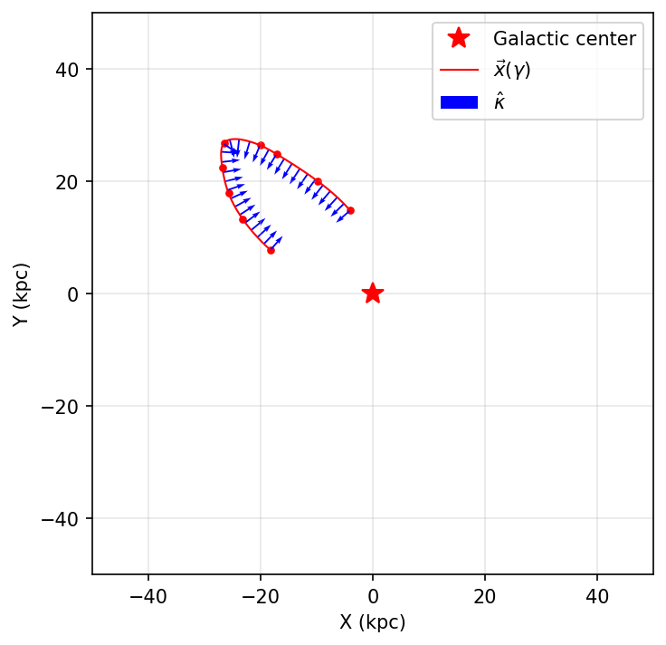
Step 1: Load Stream Data#
We use the same StreamB data from Nibauer et al. (2023):
# Example: manually extracted from Nibauer et al. (2023), Figure 5, second panel
xy = np.array([[-18.23818192,   7.7713813 ],
               [-23.20527332,  13.30501798],
               [-25.68881901,  17.85818509],
               [-26.82711079,  22.51483327],
               [-26.51666758,  26.81189831],
               [-20.04832301,  26.39824245],
               [-17.02861664,  24.77713165],
               [ -9.74451624,  19.97321842],
               [ -4.03009244,  14.80896887]])

print(f"Stream contains {len(xy)} control points")
Stream contains 9 control points
Step 2: Create Spline Track#
Parameterize the stream using arc-length:
def make_gamma_from_data(data):
    """Compute normalized arc-length parameter gamma ∈ [-1, 1]"""
    s = splinelib.point_to_point_arclength(data)
    s = jnp.concat((jnp.array([0]), s))
    s_min = s.min()
    gamma = 2 * (s - s_min) / (s.max() - s_min) - 1
    return gamma

gamma = make_gamma_from_data(xy)
track = ptd.Track(gamma, xy)

print(f"Track created with {len(gamma)} points")
Track created with 9 points
Visualize the track:
fig, ax = plt.subplots(figsize=(5, 5), dpi=150)
plt.plot(0, 0, 'r*', markersize=12, label='Galactic center')
plot_sparse_gamma = jnp.linspace(-1, 1, num=30)
track.plot_all(plot_sparse_gamma, ax=ax, show_tangents=False)
ax.set_xlabel("X (kpc)")
ax.set_ylabel("Y (kpc)")
ax.set_xlim(-50, 50)
ax.set_ylim(-50, 50)
ax.set_aspect('equal')
ax.legend()
ax.grid(alpha=0.3)
plt.tight_layout()
plt.show()
Step 3: Define Potential Model and Likelihood#
Set up the gravitational potential and likelihood computation:
# Default potential parameters
params_defaults = {
    "rs_halo": 16,
    "vc_halo": u.Quantity(250, "km/s").ustrip("kpc/Myr"),
    "q1": 1.0,
    "q2": 1.0,  # ← Will be fitted
    "q3": 1.0,
    "phi": 0.0,  # ← Will be fitted
    "origin_x": 0, "origin_y": 0, "origin_z": 0,
    "Mdisk": 5e12,
    "rot_z": 0.0, "rot_x": 0.0,
}
params_statics = {"withdisk": False}

@jax.jit
def compute_acc_hat(params, pos2d):
    """Compute unit acceleration vectors."""
    pos3d = jnp.zeros((len(pos2d), 3))
    pos3d = pos3d.at[:, :2].set(pos2d)
    merged = params_defaults | params_statics | params
    merged["origin"] = jnp.array([
        merged.pop("origin_x", 0),
        merged.pop("origin_y", 0),
        merged.pop("origin_z", 0),
    ])
    return ptd.compute_accelerations(pos3d, **merged)

@jax.jit
def compute_ln_likelihood_scalar(params, pos2d, unit_curvature, where_straight=None):
    """Compute normalized log-likelihood for a parameter set."""
    unit_acc_xy = compute_acc_hat(params, pos2d)
    where_straight = (
        where_straight if where_straight is not None
        else jnp.zeros(len(unit_curvature), dtype=bool)
    )
    lnlik = ptd.compute_ln_likelihood(
        unit_curvature, unit_acc_xy, where_straight=where_straight
    )
    return lnlik

compute_ln_likelihood = jax.vmap(
    compute_ln_likelihood_scalar, in_axes=(0, None, None, None)
)

print("✓ Likelihood functions defined and JIT compiled")
✓ Likelihood functions defined and JIT compiled
2D Parameter Sampling#
Key change from 1D inference: We now define two parameters in the
ranges dictionary instead of one.
Parameter interpretation:
q2 ∈ [0.1, 1.0]: y-axis flattening
q2 = 1.0 → spherical
q2 < 1.0 → oblate (flattened)
Note: We use the standard range (0, 1] following common practice in recent literature
phi ∈ [0, π/2]: Orientation of the halo’s long axis in the x-y plane (radians)
phi = 0 → aligned with x-axis
phi = π/2 → aligned with y-axis
# Define 2D parameter range
ranges = {
    "q2": (0.1, 1.0),     # y-axis flattening parameter
    "phi": (-jnp.pi/2, jnp.pi/2),  # Orientation angle [rad]
}

# Generate uniform random samples
key = jr.key(0)
skeys = jr.split(key, num=len(ranges))
nsamples = 1_000

params = {
    k: jr.uniform(skey, minval=v[0], maxval=v[1], shape=(nsamples,))
    for skey, (k, v) in zip(skeys, ranges.items(), strict=True)
}

print(f"Sampling {nsamples} points in 2D parameter space")
print(f"  q2 range: [{ranges['q2'][0]}, {ranges['q2'][1]}]")
print(f"  phi range: [{ranges['phi'][0]:.2f}, {ranges['phi'][1]:.2f}] rad")

# Compute likelihood for all samples
lnlik_seg = compute_ln_likelihood(
    params,
    track(gamma),
    track.curvature(gamma),
    None,
)

print(f"✓ Likelihood calculation complete")
print(f"Log-likelihood range: [{jnp.min(lnlik_seg):.3f}, {jnp.max(lnlik_seg):.3f}]")
Sampling 1000 points in 2D parameter space
  q2 range: [0.1, 1.0]
  phi range: [-1.57, 1.57] rad
✓ Likelihood calculation complete
Log-likelihood range: [1.258, 7.440]
Visualization#
Create a 2D contour plot showing the likelihood distribution in (q2, phi) space:
# Create figure
fig, ax = plt.subplots(figsize=(6, 6), dpi=150)

# Configure 2D histogram/contours
hist2d_kw = {
    "bins": 30,
    "levels": [0.95],
    "plot_contours": True,
    "plot_datapoints": False,
    "smooth": 1.0,
}

# Plot 2D likelihood contours
corner.hist2d(
    params["q2"],
    params["phi"] * 180 / jnp.pi,  # Convert to degrees
    weights=np.exp(lnlik_seg - lnlik_seg.max()),
    ax=ax,
    color="purple",
    plot_density=True,
    contourf_kwargs={"cmap": "Purples", "vmin": 0, "vmax": 1},
    **hist2d_kw,
)

# Format axes
ax.set_xlim(0.1, 1.0)
ax.set_ylim(-90, 90)
ax.set_xlabel("q₂ (y-axis flattening)", fontsize=12)
ax.set_ylabel(r"φ [deg] (orientation)", fontsize=12)

# Create legend
legend_elements = [
    Line2D([0], [0], color="purple", linestyle="-", linewidth=2,
           label=r"95% credible region"),
]
ax.legend(handles=legend_elements, loc="upper right", fontsize=10)

ax.grid(alpha=0.3)
plt.tight_layout()
plt.show()
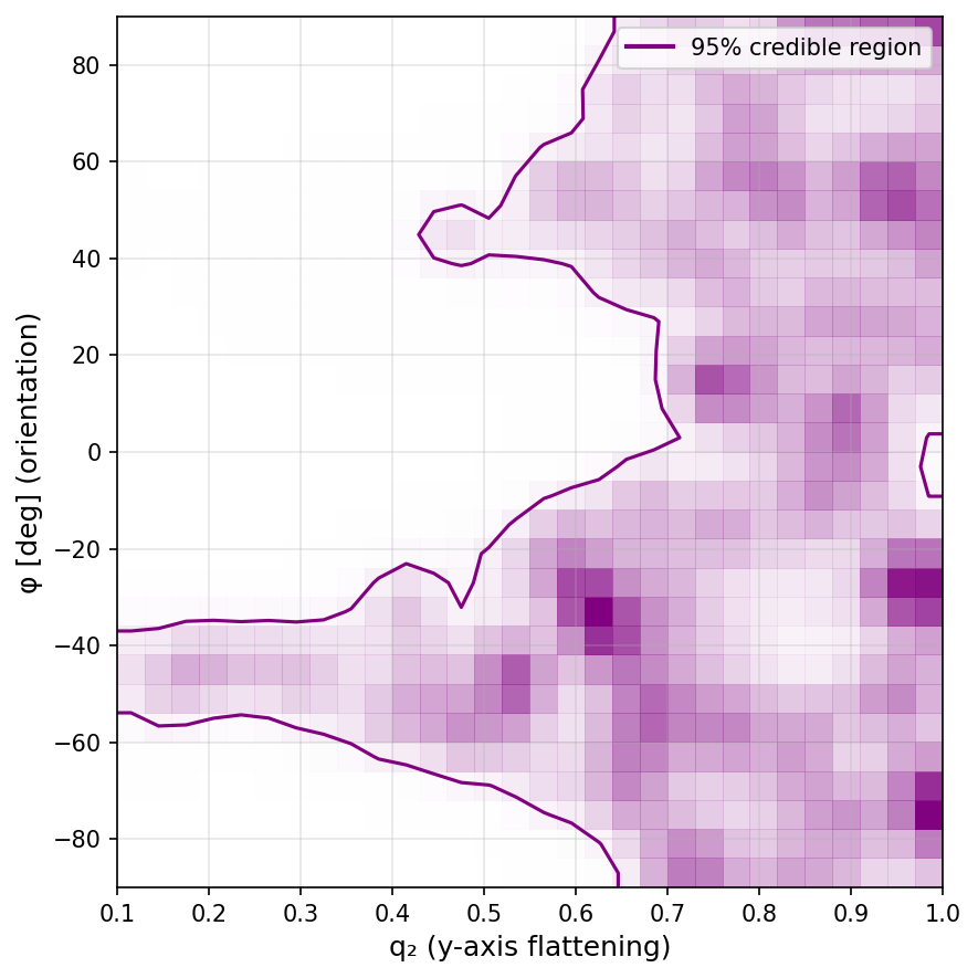
Interpretation#
The purple shaded region in the contour plot represents the 95% credible region where the model parameters are consistent with the observed stream curvature.
Key characteristics of this likelihood function:
Step-like behavior: The likelihood function is relatively flat within the credible region, meaning all parameter combinations in the purple area are nearly equally probable
Exclusion-based inference: Rather than pinpointing a unique best-fit solution, this method is most effective at ruling out incompatible parameter space
Parameters outside the purple region produce stream curvatures inconsistent with the data
Parameters inside the purple region are all compatible with observations
Physical interpretation:
The extended credible region reflects inherent degeneracies between halo flattening (q₂) and orientation (φ)
Multiple (q₂, φ) combinations can produce similar stream curvatures, making it difficult to distinguish them based on curvature alone
Additional constraints (e.g., proper motions, radial velocities, or multiple streams) are needed to break these degeneracies and narrow down the parameter space further